

The Potential of Ethanol
On this page we discuss two key factors that will enable ethanol to grow to a much larger market than has been the case to date. The first is that for engines that are designed around it, ethanol can provide more power and better mileage than gasoline. (We discuss current engines and their performance on ethanol here.) Second is that ethanol can be much more widely and cost effectively distributed if a pipeline infrastructure is built.
We will talk about both the american and Brazilian experience. But without any question the Brazilians are moving ahead faster. The plot below shows the expected increase in vehicles of different fuel types. Flex fueled vehicles, in in Brazil this means much more flexible than we have (i.e., any proportions of either hydrous or anhydrous ethanol or gasoline can be in the tank), are going to be in the vast majority.
The main handcuffs hampering the US experience is the blending limitation to 10% vs. Brazilian 25%, the refusal the auto companies to build and warranty vehicles for blends greater than 10% (whereas in Brazil the same companies build fully flex-fueled vehicles), and the lack of pipeline infrastructure (which is growing rapidly in Brazil). We will examine these below.
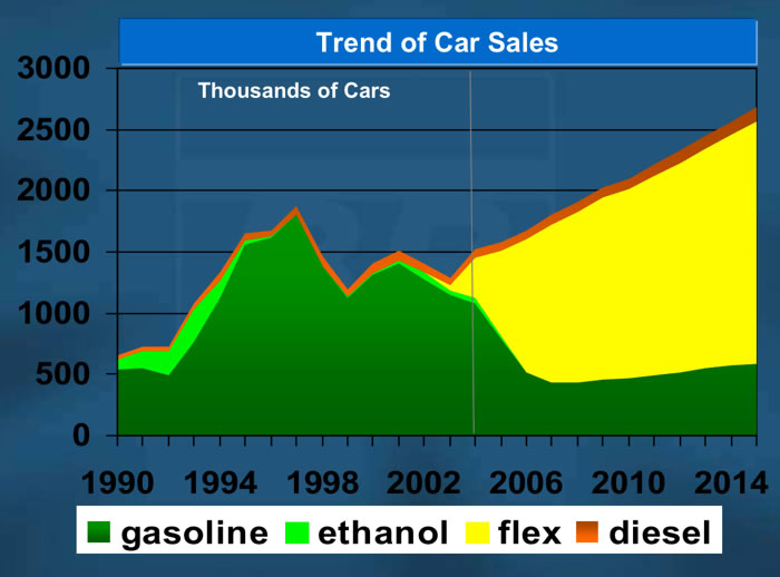 The Brazilian projections for the the sale of vehicles is shown in the plot to the right. Sales of the fully flex fuel capable vehicles is show in yellow.
1. The Power and Mileage Potential of Ethanol in IC Engines
We show, that if ethanol is allowed to give us its maximum benefits, we can all gain both more power and more mileage at a lower price.
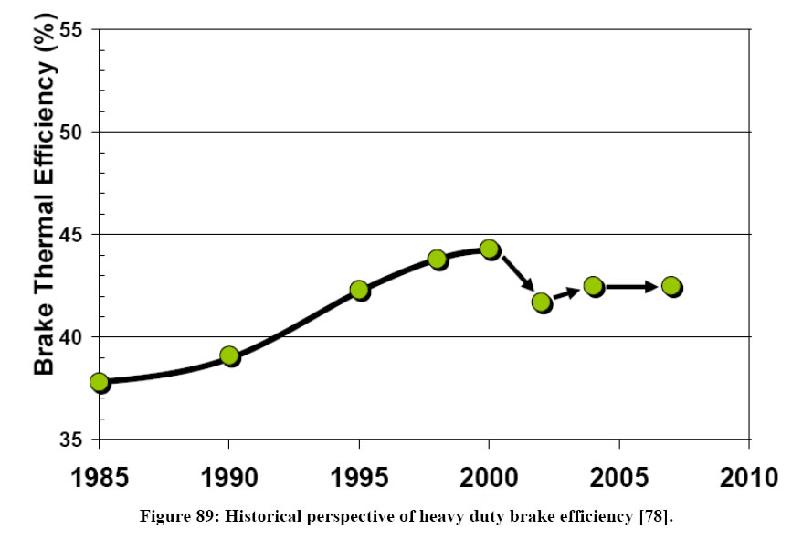
But first we want to point out that in our attempt to reduce emissions in heavy duty engine applications the steady increase in efficiency which ran up to 44.5% in 2000 has dropped to 41.5 in ensuing years (figure below). This certainly runs counter to our need to reduce both fuel consumption and GHG.
Looking for solutions, we investigate the possibilities adding ethanol to gasoline can give us.
Then we investigate the further possibilities of using hydrous ethanol vs. anhydrous ethanol, i.e., wet vs. dry ethanol.
The information in the following Sections 1.1.- 1.3. is from Stein, Polovina, Roth, Foster, Lynskey, Whiting, Anderson, Shelby, Leone, and Vander-Grien, 2012, SAE 2012-01-1277.
1.1. Thermal Efficiency of Anhydrous Ethanol Blends
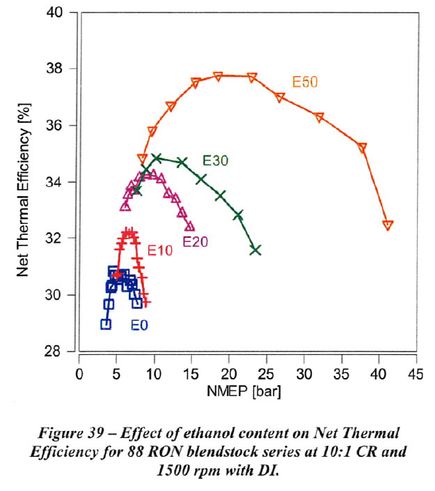
Net thermal efficiency (NTE) for the B88 fuel series at 10:1 compression ratio (CR) at 1500 rpm with DI is shown in Figure 39. As shown, the peak Net Thermal Efficiency (NTE) and the Net Mean Effective Pressure (NMEP) at which the peak NTE occurs increase substantially with increasing ethanol content. For example, peak NTE improves from 31% at 5 bar NMEP with B88EO-R93 to 38% at 20 bar NMEP with B88E50-R105 (The fuel designation convention used in this paper is as follows: the Research Octane Number (RON) of the gasoline blendstock, followed by the ethanol percentage, followed by the measured RON value; for example, B88E10-R93 designates a gasoline blendstock of 88 RON with 10% added ethanol by volume with a measured RON value of 93 for the mixture.
A large fraction of this increase in NTE is due to the higher NMEP which is achieved at a given Crank Angle (CA50) combustion phasing, and the associated reduction in pumping work and heat transfer losses per unit mass. Thus, this large increase in NTE is not representative of the overall thermal efficiency improvement which would be expected during a vehicle drive cycle which encompasses loads where optimum combustion phasing can be maintained.
Obviously, we want to run our engines at their peak thermal efficiency to get the best use of the fuel we put in. As we see in the next section, this definitely gives us the best mileage.
Another way to look at the better performance possible using ethanol is discussed on our page "Flex-Fueled Vehicles Around the World", here.
1.2. Fuel Consumption
Net specific fuel consumption (NSFC) for the data shown above is shown in Figure 40. As ethanol content is increased, improved thermal efficiency provides an offset to the reduced heating value per mass of ethanol. As shown, E20 results in the lowest minimum NSFC, while the minimum values for E10, E30, and E50 are comparable to that of EO. For this 10:1 CR engine (certainly in the range of many current vehicles on the road), first we see that E10 fuel consumption is the same as E0, and that blends with E20 are have 3% [(267.5-259)/267.5] lower fuel consumption. This ties in with the experimental values of the vehicles in section on the Value of Ethanol, although as we see there, the way the overall systems are tuned for each vehicle obviously can shift the mileage increase to be somewhere between E20 and E30.
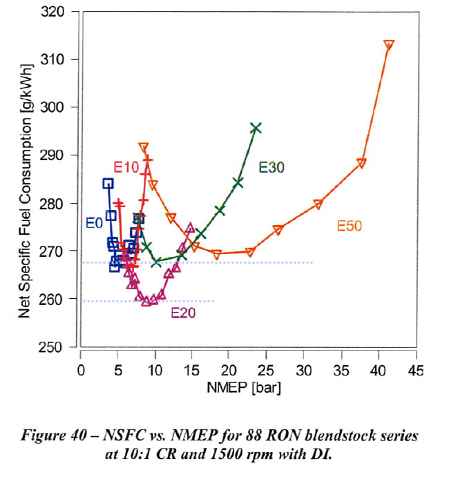
We can see that the minimums in fuel consumption occur at NMEPs where the Net Thermal Efficiencies, Fig 39 in the last section, were highest. If we can achieve these NMEPs without knocking, we would get our best gas mileage.
On the other hand, if we wanted more power, say for acceleration, it would be desirable to increase the NMEP to higher levels. Again, we could only do this if our fuel would allow it without causing knocking. We will see below the the additional of ethanol to gasoline is a very good way to achieve the higher NMEPs.
Manente 2010 showed that the normalized gross specific fuel consumption of ethanol is much less than gasoline, and diesel.
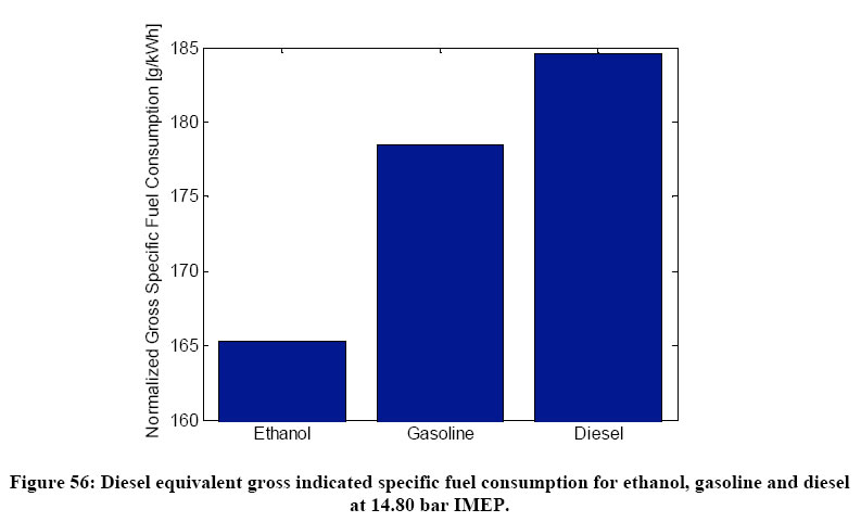
The reason this is happening is that gasoline and diesel are burning in diffusion controlled mode while with ethanol a significant amount of kinetically controlled combustion is followed by a diffusion combustion tail. As shown in many HCCI papers kinetically controlled combustion has the main advantage of fairly high thermal efficiency which leads to high indicated efficiency (low fuel consumption) as compared to classical mixing controlled or flame propagation combustion processes.
1.3. Reasons for the improved thermal efficiency and lower fuel consumption when using ethanol
The research engine used at the right, is a state-of-the-art automotive design with high tumble intake ports. The engine structure supports a 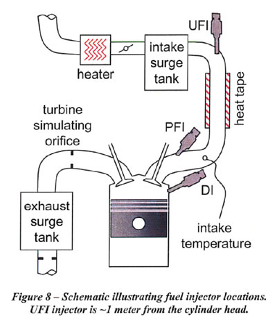 peak cylinder pressure (mean + 3 sigma) of 160 bar, which is required to determine the knock limit of the high ethanol blends. The engine is equipped with both direct injection (DI) in the side location and port fuel injection (PFI). The fuel targeting and spray pattern were validated for both the Dl and PFl fuel systems. In addition, the capability to supply fuel upstream in the heated intake piping was added in the test cell, and this is termed "upstream fuel injection" (UFI) in this paper. UFI is pre-vaporized. The UFI simulates carbureted fuel intake. A schematic of the single cylinder engine showing the fuel injector locations is shown in Figure 8.
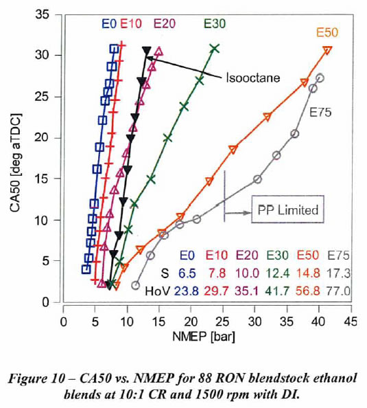
This engine allowed the effect of ethanol percentage on knock limit with direct injection at 10:1 CR and 1500 rpm with 88 RON gasoline to be determined. As shown in Figure 10 below, the low ethanol content fuels exhibit a very steep slope of Crank Angle vs. knock-limited NMEP. This plot is the result of changing the the inlet pressure at constant engine speed, and determining the spark timing that gave borderline knocking at each inlet pressure. The resulting combustion phasing, as measured by the location of 50% mass fraction burned in degrees aTDC (CA50), was plotted as a function of the 720°-based Net Mean Effective Pressure (NMEP). (aTDC means after Top Dead Center.) In this plot each line represents that spark timing giving borderline knock as the inlet pressure was increased for E0, E10, E20, E30, E50, E75 and isooctane (100 RON and 100 MON).
As ethanol content increases, the slope of CA50 vs. NMEP tends to decrease. As the slope decreases, the NMEP achievable at a given CA50 is higher. Thus, at lower CA50 values we achieve higher NMEPs. For example, NMEP increases only 4 bar as CA50 is retarded from 4 deg after Top Dead Center (aTDC) to 30 deg aTDC with B88EO-R88 fuel. B88E10- R93 and isooctane have a similar slope. However, NMEP increases by 32 bar for the same change in CA50 with B88E50-R105 fuel. This change in slope is a consequence of increasing HoV and sensitivity as ethanol content is increased.
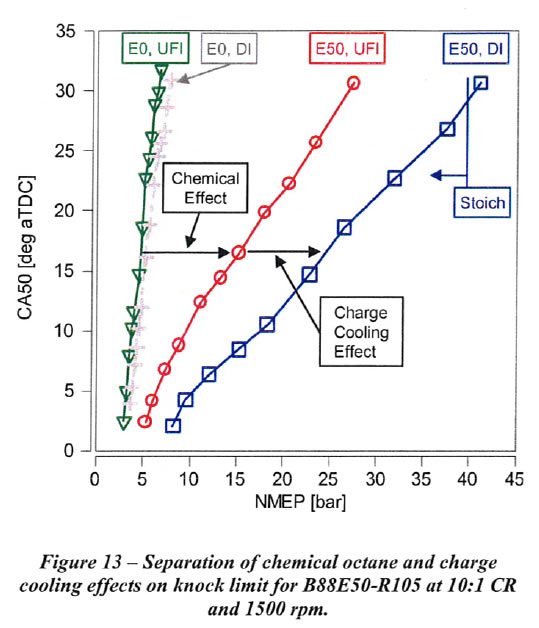
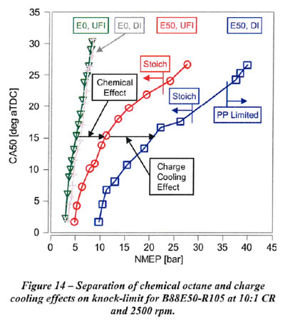
1.3.1. Separating Out the Charge Cooling Effects of Ethanol
Separation of the chemical octane and charge cooling effects on the knock-limited NMEP for E50 compared to EO with 88 RON gasoline blendstock is shown in Figures 13 and 14 for 1500 rpm and 2500 rpm, respectively. The knock-limited NMEP increase from UFI with EO to UFI with E50 is attributed solely to the higher chemical octane of E50, since it is assumed that the fuel for UFI is fully vaporized. The knock-limited NMEP increase from UFI to Dl for each fuel is attributed to charge cooling due to vaporization of the fuel in the cylinder with Dl. Charge cooling results in a small increase in NMEP for EO. The increase for E50 is much greater than for EO as a consequence of the higher heat of vaporization (HoV) and sensitivity of E50 compared to EO. As shown in Figures 13 and 14, both the chemical octane and charge cooling effects for B88E50-R105 fuel are very significant. The reduction in the slope of CA50 vs. knock-limited NMEP for UFI with ES0 is due to the high sensitivity of the auto ignition kinetics of ethanol to unburned gas temperature. The further reduction in slope for E50 with Dl is due to the additional reduction in unburned gas temperature with charge cooling, and the consequent effect on auto ignition kinetics with high fuel sensitivity.
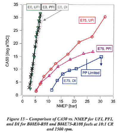
PFI (port fuel injection), used on the majority of vehicles on the road today, is anticipated to result in a charge cooling effect which is between that of Dl (Direct Injection) and UFI. Results for PFI compared to DI and UFI are shown in Figure 15 for EO and E75 with B88 gasoline blendstock. As shown, Dl provides a small benefit relative to UFI with B88EO-R88 fuel, and PFI performs similar to UFI. Thus, sadly the use of DI or PFI and E0 gain us nothing over the 'carbureted' tests.
With B88E75-R108 fuel (with much greater HoV), PFI initially performs similarly to UFI at advanced CA50. As NMEP and fuel flow increase, PFI improves relative to UFI. Initially perhaps a large portion of the HoV of the fuel with PFI comes from the intake port and valves, whereas at higher NMEP, increased fuel flow with Open Valve Injection (OVI) timing results in increased charge cooling. For higher NMEP it is clear that ethanol helps all of the forms of fuel injection, with PFI still being better than UFI and DI being the best.
2. Effect of Ethanol Content on RON Kept Constant by Lowering Blendstock Quality - Reasons Why We Don't See the Value of Ethanol
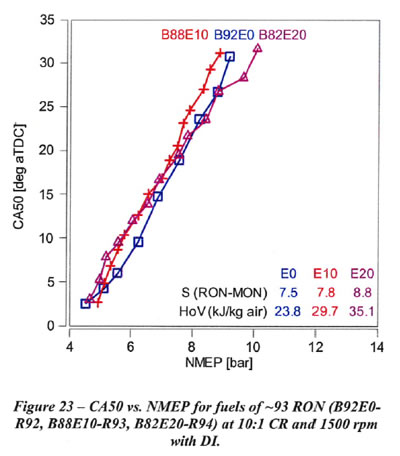
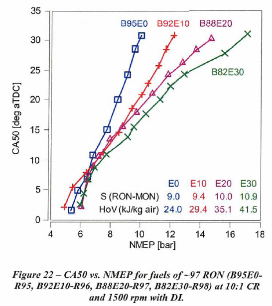
Figures 23 shows CA50 vs. knock-limited NMEP for fuels of approximately constant RON values of 93. the octane 93 RON fuels which range from EO to E20 shown in Figure 23 perform similarly for all CA50 values. Note in Figure 23 that the sensitivity is nearly constant, and only the E20 fuel (with the highest HoV) shows a slight reduction in slope.This is the situation refineries have made for us for the last two decades, because they do not want to give us 'free value'. However, if they persist with their business model, we may still get a little value out of blending to E20.
However, if the blendstock enables a RON of 97, increasing ethanol content significantly increases the knock-limited NMEP at retarded CA50, which range from EO to E30. If refineries would go back to their early 1980s practice, we could once again enjoy the higher thermal efficiency and better mileage ethanol blends can provide.
3. Hydrous vs. Anhydrous Ethanol in IC engines
Anhydrous ethanol means an ethyl alcohol that has a purity of at least ninety-nine percent, exclusive of added denaturants, that meets all the requirements of the American Society of Testing and Materials (ASTM) D4806, the standard specification for ethanol used as motor fuel. Hydrous (or wet) ethanol is the most concentrated grade of ethanol that can be produced by simple distillation, without the further dehydration step necessary to produce anhydrous (or dry) ethanol. Hydrous ethanol (also sometimes known as azeotropic ethanol) typically ranges from 186 proof (93% ethanol, 7% water) to 192 proof (96% ethanol, 4% water).
Initial tests conducted in Europe have confirmed that hydrous ethanol can be blended effectively with gasoline without phase separation or other problems. An unmodified Volkswagen Golf 5 FSI was operated successfully on HE15 (15% hydrous ethanol blended with gasoline), meeting European exhaust emission standards in testing conducted by the Netherlands research organization TNO Automotive and by SGS Drive Technology Center of Austria. In addition to confirming the effectiveness of hydrous ethanol for gasoline blending in actual vehicle trials, these initial tests have shown measurable increases in volumetric fuel economy, indicating higher thermodynamic efficiencies resulting from hydrous ethanol. This recently discovered phenomena for mid-level ethanol blends appears to be due to the benefits of oxygenation and heat of vaporization in conjunction with capitalizing on the change in chemical and physical properties which occur as a result of combining water, ethanol, and gasoline. When appropriately combined in mid-level ethanol blends, the chemical reactions of these compounds optimize the efficiency at which internal combustion engines operate. For hydrous ethanol blends, this is accomplished primarily through the total heat of vaporization resulting from combining ethanol and water. Essentially, the lower energy content of hydrous ethanol is counteracted by increasing engine performance due to higher heat of vaporization of ethanol and water in comparison with gasoline and anhydrous blends.
Hydrous ethanol blends (oxygenated hydrocarbons) lower engine operating temperatures due to cooling of intake fuel mixture with 3-6% more water and increasing heat of vaporization when compared to anhydrous ethanol. The result is more efficient combustion, cooler running engines, lower exhaust temperatures, and increased longevity of engine life. The water contained in hydrous ethanol blends also reduces NOx emissions. In addition to the effects of higher water content in hydrous ethanol, ethanol increases compression ratios and decreases engine knocking (detonation). Essentially, both water and ethanol increase the octane level of the fuel mixture. The octane number is a measure of the resistance of a fuel to auto-ignition. It is also defined as a measure of anti-knock performance of a gasoline or gasoline component such as hydrous ethanol. Higher octane levels contribute to enhancing the thermodynamic efficiency of combustion engines, which subsequently increases fuel efficiency. The increase in total engine efficiency results in optimizing fuel efficiency for both ethanol and gasoline.
Previous assumptions held that ethanol’s lower energy content directly correlates with lower fuel economy for automobiles. Those assumptions were found to be incorrect. Instead, the new research strongly suggests that there is an “optimal blend level” of ethanol and gasoline – most likely E20 or E30 – at which cars will get better mileage than predicted based strictly on the fuel’s per-gallon Btu content. The 2007 flex-fuel Chevrolet Impala utilized in midlevel blends testing revealed a 15% increase in fuel efficiency using the Highway Fuel Economy Test (HWFET) for E20 in comparison with unleaded regular gasoline. For the same vehicle, the highway fuel economy was greater than calculated for all tested blends, with an especially high peak at E20. The new study, co-sponsored by the U.S. Department of Energy (“DOE”) and the American Coalition for Ethanol (“ACE”), also found that mid-range ethanol blends reduce harmful tailpipe emissions.
Flex-Fuel vehicles were launched in the Brazilian market in 2003. They can operate with gasohol (gasoline blended with 18–25% vol/vol anhydrous ethanol), 100% hydrous ethanol (4.0– 4.9% vol/vol of water) or any blend of these fuels. This technology is well accepted in the country, representing over 80% of the total number of new vehicles sold in Brazil since 2009.
According to Baylor University, “as far as safety and performance is concerned, hydrous ethanol is a slightly better fuel [than anhydrous ethanol] in every respect (except specific fuel consumption since water does not provide any caloric content). Small quantities of water absorbed in the fuel result in a slight increase in power caused by the higher latent heat of vaporization of the fuel.”
Hydrous (or wet) ethanol is also used in Holland and Sweden. It has a number of advantages over anhydrous ethanol, discussed above -- which is largely used in the US.
4. Distribution and storage of hydrous vs. anhydrous ethanol
Because hydrous ethanol has water bonded to it, it has much less of a tendency to attached additional water to it. A result is that it can be distributed in petrol pipelines with less difficulty. This enormous advantage over anhydrous ethanol may significantly enhance its presence around the country and the world.
In this section we discuss Brazilian distribution and storage of both hydrous and anhydrous ethanol. We especially note that the ethanol pipeline infrastructure is rapidly expanding in Brazil, and that there is no reason why ethanol distribution via pipeline could not be used to more widely and cheaply distribute midwestern ethanol.
4.1. Brazilian ethanol pipeline infrastructure
Brazilians have been using pipelines to distribute ethanol for many years. Existing annual flows are indicated below (from 2000-2006).
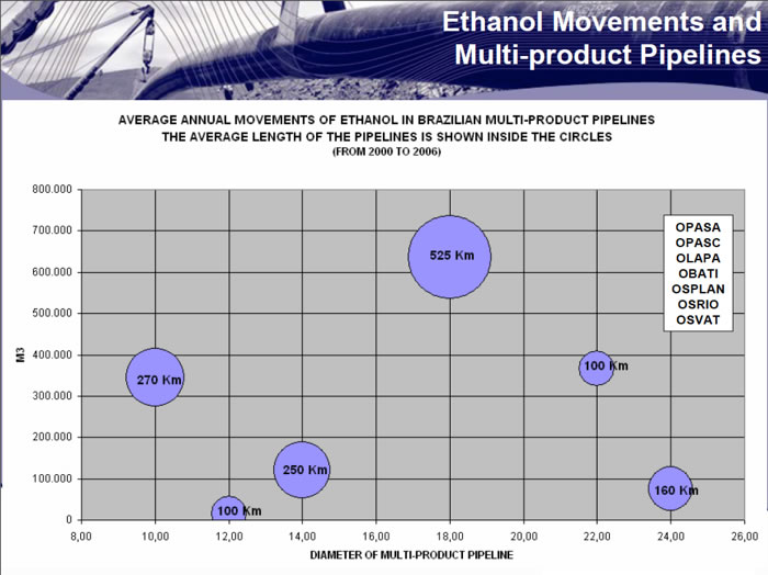
But it is well understood that more pipelines will help distribution and further spur exports.In 2008 only 19% of Brazilian ethanol moved in multi-product pipelines.
![]()
The map below shows existing and planned pipelines in 2007.
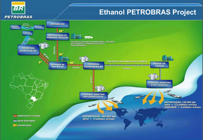
These are further quantified below.
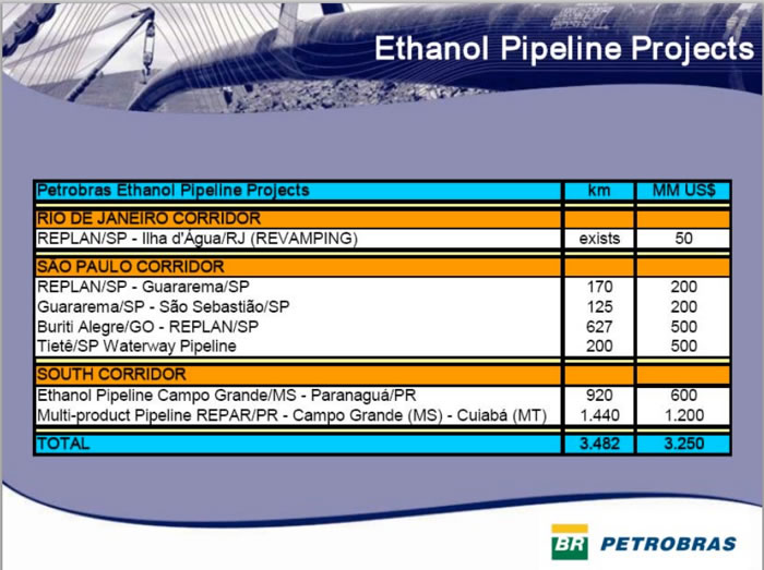
Since 2004, PETROBRAS has built 2 additional ethanol pipelines by 2012: a 1,150-km-long pipeline from Buriti Alegre (Goiás State) to the Port of São Sebastião (State of São Paulo) and a 525-km-long pipeline from Minas Gerais to the port in Rio de Janeiro. The new pipelines will allow for the transport of about 8 billion liters of ethanol at a cost of R$0.04, compared with the current R$0.13 per liter by truck (VEJA, 2007).
Thus, ethanol pipelines result in transport costs of less than 1/3 of truck and rail.
What about the US suggestions that Stress Corrosion Cracking and Corrosion in general are major issues in ethanol pipelines? Well, many years of engineering in Brazil have long ago solved these problems. As the slide below from the US DOT relays:
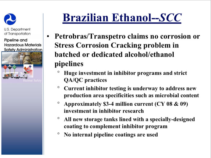
So why are we in the US not moving ethanol in pipelines? Ask your congressperson.
4.2. US dedicated ethanol pipeline status
As in Brazil's case, successfully integrating ethanol into the national fuels portfolio requires investment throughout the supply chain. For blending operations, both ethanol and gasoline must be at the delivery points in the quantities needed to reliably sustain a continuous supply. Attaining this essential balance requires careful judgment as to where and when to invest in fixed assets such as pipelines, ports, rail facilities, and terminals. These decisions require a reasonable degree of certainty about future patterns of biofuels supply and demand.
A report to congress entitled "Dedicated Ethanol Pipeline Feasibility Study by DOE 2007, concludes:
"Ethanol Volume Requirements: Based on current consumption projections, the ethanol volume likely to be transported by a dedicated pipeline from the Midwest to the East Coast was determined to be approximately 2.8 billion gallons per year (bgy) over the asset’s 40-year lifespan. This projection includes demand from low-level ethanol blends (10 percent ethanol, 90 percent gasoline or E10) used in conventional vehicles and high-level ethanol blends (85 percent ethanol, 15 percent gasoline or E85) used in flexible fuel vehicles (FFVs). Even with the financial incentives considered here, this volume is not sufficient to make the pipeline competitive with current modes of distribution (rail, barge, and truck)."
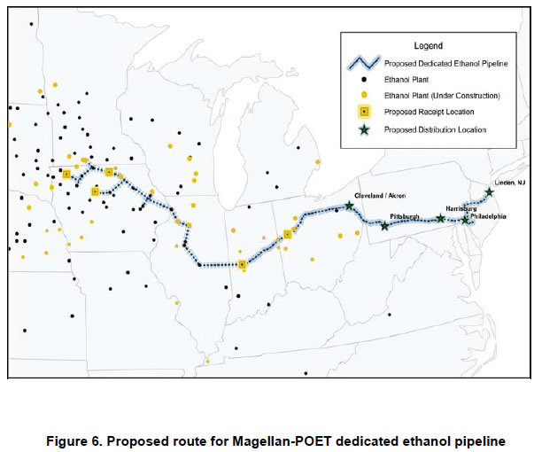
"For the pipeline to be economically viable without major financial incentives, it would need to transport approximately 4.1 billion gallons of ethanol per year—a volume that exceeds projected demand in the target East Coast service area by 1.3 bgy. This level could be achieved in this region with a significant increase in demand for E85 and/or the widespread use of ethanol blends greater than 10 percent if an increase in the percent ethanol allowed for blending in motor gasoline is approved by the Environmental Protection Agency (EPA). Based on the assumed ethanol demand volume (2.8 bgy) and a project construction cost of $4.25 billion, the pipeline would need to charge an average tariff of 28 cents per gallon, substantially more than the current average rate for ethanol transport across current modes (rail, barge, and truck) along the same corridor (19 cents per gallon). Even at a lower pipeline construction cost iv ($3.75 billion), significant financial incentives would be required to make the pipeline profitable if ethanol blends remain capped at 10 percent and E85 demand is not significantly expanded." The proposed route is shown below."
"Technical challenges associated with a dedicated ethanol pipeline involve pipeline integrity as well as fuel delivery and consumption issues. Addressing these issues will require continued study of stress corrosion cracking (SCC) to improve pipeline integrity and development of an internal SCC diagnostic tool for pipeline maintenance. The DOT is addressing pipeline safety and integrity threats through a comprehensive research program that will drive new knowledge into industry best practices and consensus standards."
Compatibility associated with the potential use of the ethanol pipeline for a variety of non-ethanol biofuels including green gasoline and diesel should also be evaluated as a potential source for additional fuel volumes for transport. In an effort to remove technical barriers to increased market demand, existing fleet vehicle studies are examining system compatibility with blends above E10.
The report concludes: "that in spite of the documented challenges and risks, a profitable, dedicated ethanol pipeline is feasible under certain scenarios. A pipeline would enhance the fuels delivery infrastructure, reduce congestion of rail, truck, and barge transportation, and would reduce greenhouse gas emissions when compared to current delivery methods. The faster product delivery cycles, more reliable delivery schedules, and increased safety will enhance the flexibility to accommodate any significant expansions in ethanol production and demand in the future."
5. Sugarcane crop improvements
There are several areas being addressed in sugarcane growth that will make sugar cane harvest yield more ethanol.
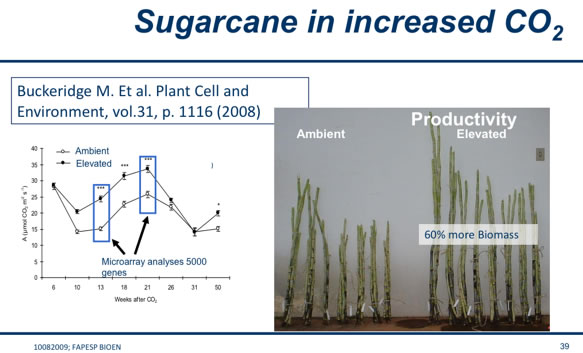
5.1. Understanding how the changes in CO2 effect sugarcane
While we all know that plants use CO2, it is still impressive how CO2 can increase the biomass of sugarcane. The study by Buckeridge et al. shows 60% more biomass resulting.
.